Exploring the parameters of convolutional neural networks to create an accurate image classifier.
Final GitHub Repo: EECS349_Project
Contributors: Adam Pollack, Chainatee Tanakulrungson, Nate Kaiser
Summary
The objective of this project was to predict the presence of lung cancer given a 40×40 pixel image snippet extracted from the LUNA2016 medical image database. This problem is unique and exciting in that it has impactful and direct implications for the future of healthcare, machine learning applications affecting personal decisions, and computer vision in general. The medical field is a likely place for machine learning to thrive, as medical regulations continue to allow increased sharing of anonymized data for the sake of better care. Not only that, but the field is still new enough that our project implements methods at the forefront of technology.
Approach
Due to the complex nature of our task, most machine learning algorithms are not well-posed for this project. There are currently two prominent approaches for machine learning image data: either extract features using conventional computer vision techniques and learn the feature sets, or apply convolution directly using a CNN. In the past few years, however, CNNs have far outpaced traditional computer vision methods for difficult, enigmatic tasks such as cancer detection. We decided to implement a CNN in TensorFlow, Google’s machine learning framework.
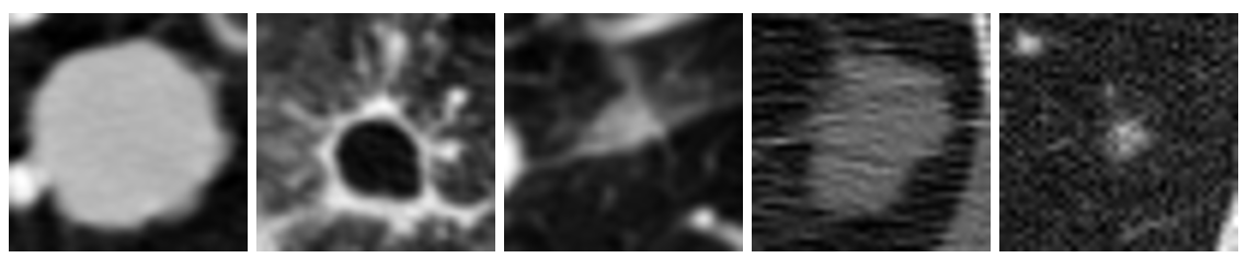
Figure 1: Examples of cancerous images
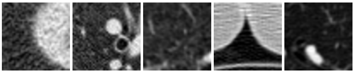
Figure 2: Examples of non-cancerous images
Because we collectively had limited experience with convolutional neural networks, we decided to first explore the hyperparameters of a CNN. We did so by creating an experiment in which we varied the kernel size and number of filters of each convolutional layer and the dropout rate for a total of 108 models. For this study, we kept a constant network architecture.
| Attribute | Values Tested |
|---|---|
| Kernel Size (Convolutional Layer 1) | 3x3, 5x5, 7x7 |
| Kernel Size (Convolutional Layer 2) | 3x3, 5x5, 7x7 |
| Number of Filters (Convolutional Layer 1) | 16, 32 |
| Number of Filters (Convolutional Layer 2) | 32, 64 |
| Dropout Rate | 0.1, 0.2, 0.3 |
Each model was trained on 2,064 images (batch size of 104), validation was run every 10 epochs on another 442 images, and a final test was run after 500 epochs on another 442 images.
Results
After determining the best set of hyperparameters based on average peak validation accuracy, we then tested six new architectures based on these hyperparameters. The structure of each of these architectures was decided based on the principles described in the Stanford CS231n course notes[1]. After running the final six architectures at 500 epochs, we found the inflection point of the loss to be around 250 epochs. We then ran each of the six architectures for 250 epochs and recorded the final test accuracy. The best network architecture of these six achieved a test accuracy of 96.38%.

Figure 3: Tensorboard Graph of Accuracy for Final Model at 500 epochs (Orange Line = Training Dataset, Blue Line = Validation Dataset)
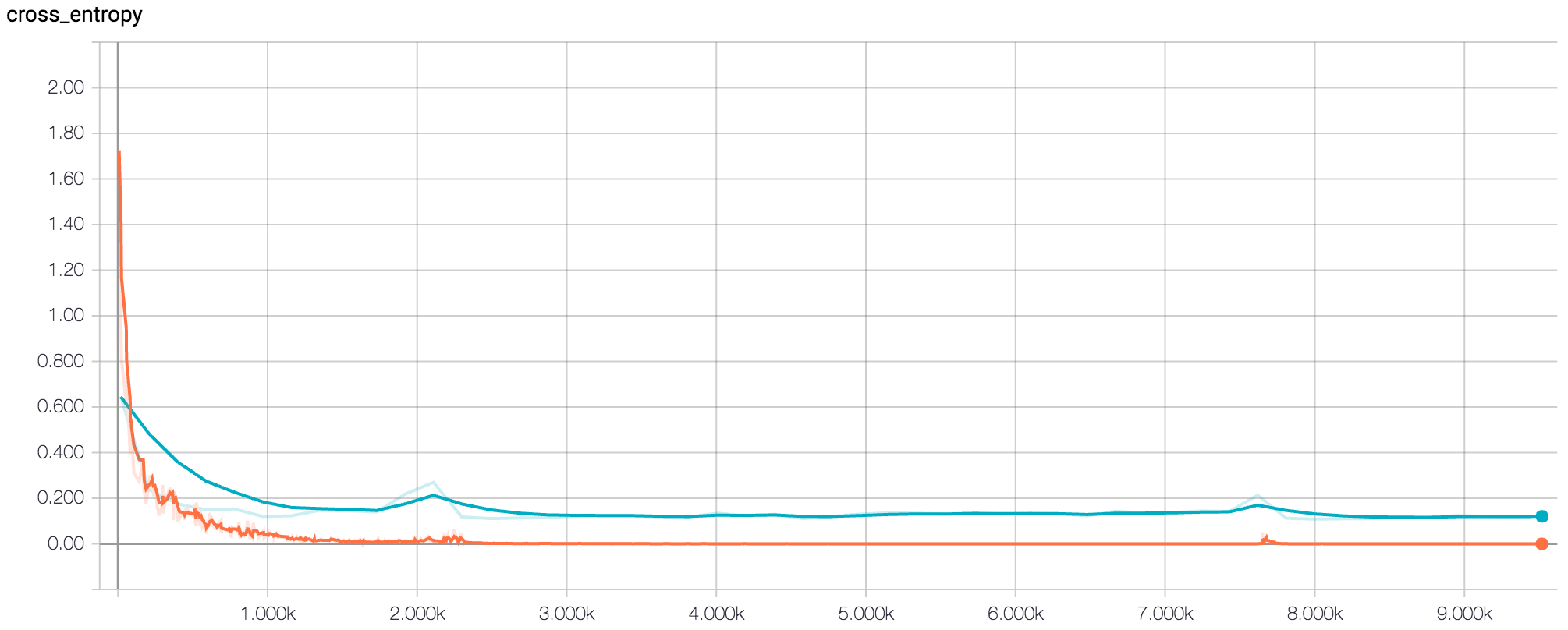
Figure 4: Tensorboard Graph of Loss for Final Model at 500 epochs (Orange Line = Training Dataset, Blue Line = Validation Dataset)
Conclusion
After finding our best model, we ran further analysis to extract a confusion matrix and misclassified images of the final test results to determine why this number was not closer to 100%.
| Predicted Positive | Predicted Negative | |
|---|---|---|
| Actual Positive | 226 | 12 |
| Actual Negative | 4 | 200 |
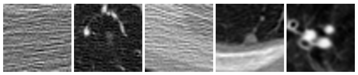
Figure 5: Examples of misclassified images from the test dataset
Our model classified more examples as negative when they should have been positive than vice versa. We believe this is because of the nature of some of the positive examples. For example, the first four misclassified images above are all positive examples of cancer even though two of them have almost no distinct features. It is likely that it would be just as difficult for a human to classify those images as a doctor. We also can’t guarantee that the data we used is completely correctly classified; it is possible there are some mislabeled images.
Future Work
We plan to test our model on entire scans of a lung by extracting 40x40 images from each image slice of the lung. Sliding a window with a stride of around 20 would give us a large set of images to test for cancer but with a pre-trained model, this would be relatively easy to do. Our hope is that this method would allow us to determine whether or not cancer is present in an entire lung instead of a predetermined section. We would also like to try implementing one or more named convolutional neural networks such as AlexNet[2] or Inception[3].
Final Report
If you are intersted in learning more about the details of this project, please read our report.
References
[1] Stanford Course Notes on CNNs: http://cs231n.github.io/convolutional-networks/
[2] AlexNet: http://papers.nips.cc/paper/4824-imagenet-classification-with-deep-convolutional-neural-networks
[3] Inception (by Google): https://arxiv.org/abs/1409.4842