Using optical flow and an extended Kalman filter to generate more accurate odometry of a Jackal robot.
Final GitHub Repo: advanced-computer-vision
In collaboration with Nate Kaiser.
Summary
We demonstrated a system which uses vision processing techniques to improve the estimation of the state of a Jackal UGV from Clearpath Robotics. We applied feature tracking, optical flow, and perspective transform to derive the estimated motion of the robot from a camera alone. This motion estimation is then combined with data from an inertial measurement unit (IMU) in an extended Kalman filter (EKF) through a process called sensor fusion in order to provide a more accurate estimation of the robot’s state. We primarily focused on solutions which are computationally cheap and can be implemented on the Jackal’s onboard computer.
Motivation
The Jackal UGV is made primarily to be an entry-level research robot which has an onboard computer, GPS, and inertial measurement unit (IMU) integrated with the Robot Operating System (ROS). The inertial measurement unit, which was the focus of our project, contains sensors which measure the orientation, angular velocity, and linear acceleration of the robot. Through our work with Jackal, we found that the IMU on board often takes noisy measurements which contain inaccuracies and drift. We wanted to develop a fully working system which could compensate for this IMU noise by utilizing an optical camera. Through only measurements from the optical camera and the IMU we sought to filter the data gathered about the odometry of the robot in order to make better predictions about its location in the real world.
Methods
Code Overview
C++/Python: For the computer vision portion, we wrote code in C++ because the algorithms we are using tend to be very computationally intensive. Python was used to perform sensor fusion, tie in functionality from ROS, and collect data when necessary. Using a combination of programming languages allowed us to code for efficiency or speed depending on the application, and with ROS, the integration of these languages was seamless.
Robot Operating System (ROS): ROS allowed us to write individual nodes which perform different computations, and then pass data easily between nodes using publishers and subscribers. We chose to use ROS because it is commonly applied to robotic systems and because we wrote our code in both C++ and Python, it enabled easier data transfer.
OpenCV: OpenCV is a commonly used computer vision library which happens to work very well with Python, C++, and ROS, so it was a great choice to handle some of our vision applications.
Feature Tracking
In order to derive motion from a video feed, we first had to determine which features we wanted to track in the image. To do this we looked into the Shi-Tomasi paper titled Good Features to Track[1]. In this paper, Jianbo Shi and Carlo Tomasi outline methods to determine which features of an image are unique enough to be identified in multiple pictures of the same scene. Figure 1 shows the results of the Shi-Tomasi Method.
Figure 1: Feature Tracking Results
Calculating Optical Flow
To calculate optical flow, we used the Lucas-Kanade Method. The Lucas-Kanade Method uses the assumption that all neighboring pixels will have similar motion to extract optical flow. Their method assigns a weight function to the pixels and then uses the Weighted Least Squares method to formulate an equation to derive motion[2].
Extracting Motion
We used perspective transform to extract motion from our optical flow data. The perspective transform method relies on relating the pixel coordinates (u, v) to world coordinates (x, y, z). This relationship is desirable because we already have the motion of the camera in (u, v) coordinates from optical flow so a simple transformation from pixel to world coordinates would provide the information we need. Finding the desired transformation required only taking some measurements relating the camera to the ground.
Sensor Fusion
Sensor fusion is the combination of measurements from multiple different sensors to create a more accurate measurement[3]. The more accurate estimation is derived using an Extended Kalman Filter based on the input measurements. Since the goal of our project is to stabilize noisy IMU data, we looked at performing sensor fusion using data from the inertial measurement unit on board Jackal and the extracted motion from our optical flow calculations above. The figure below shows the basic principle behind sensor fusion in which two sets of data (pink and red) are fused to form the estimation (green).
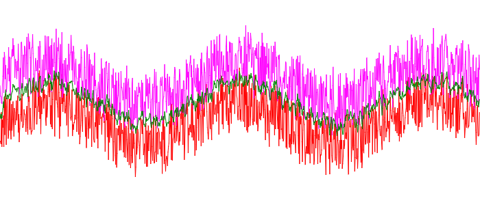
Figure 2: Sensor Fusion Example
Results
Testing Details
We gathered data for four different test cases including stationary, normal driving, aggressive driving, and random driving. The stationary test case consisted of not moving the robot. Normal driving involved driving the robot around at a medium speed and making gradual turns. Aggressive driving included forward and backward motion at the highest speed as well as some quick turns. And finally, random driving consisted of a mix between slow and fast driving and quick and slow turns. For each test, we collected odometry data from the IMU alone, the IMU fused with optical flow data, and the wheel odometry built-in to Jackal’s codebase. Below are three graphs of results we collected.
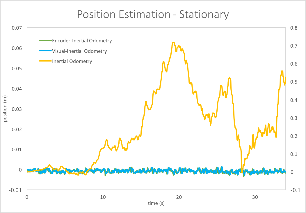
Figure 3: Stationary Position Estimation
Figure 3 shows that the visual-inertial odometry filters out almost all of the noise and drift accrued using the IMU alone. The robot is not moving, so the x-position for all three cases should show a reading very close to zero. The encoder-inertial performed as expected given that the encoders should be reading a constant, zero value for x-position. Our visual-inertial reading performed nearly identically to the encoder-inertial results which suggests that our optical flow calculations improved the IMU data.

Figure 4: Aggressive Driving Position Estimation
Figure 4 shows the position estimation for the aggressive driving test case. For this case, the IMU data has again drifted completely away from the visual-inertial and encoder-inertial odometry. However, aggressive driving also demonstrated a discrepancy between the encoder and visual odometry cases. The difference between the two results is most likely due to the inaccuracies of the encoder when the wheels are slipping and the inaccuracies of optical flow when at high speeds. The actual position is likely in between these two results.
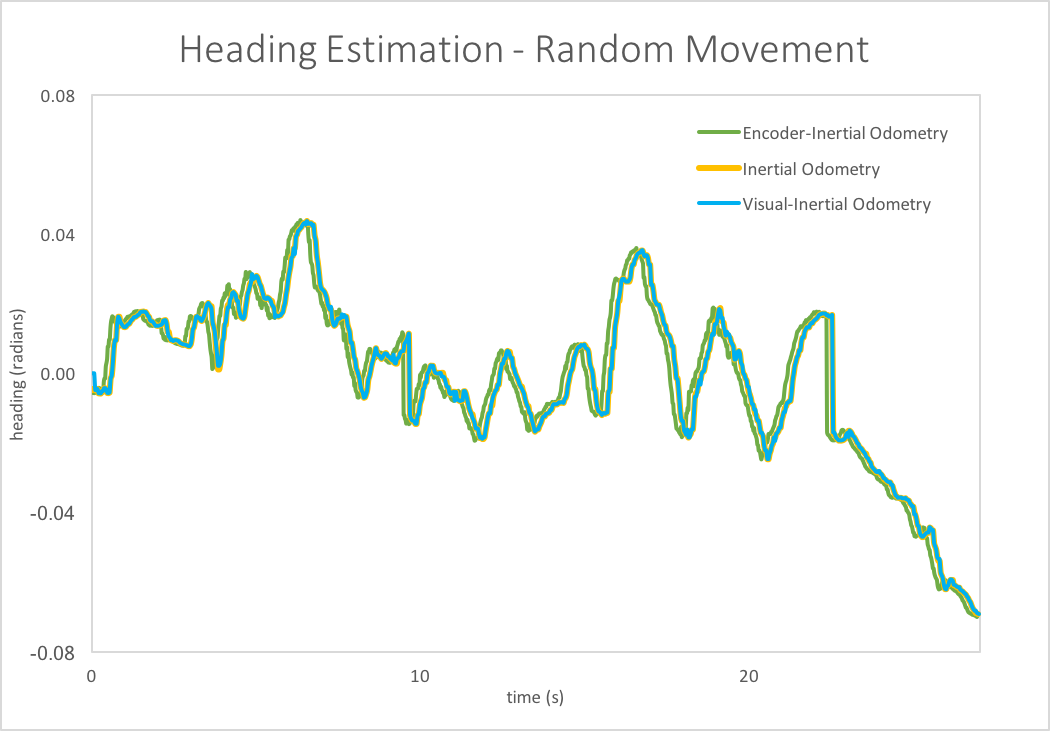
Figure 5: Random Driving Heading Estimation
Figure 5 is a graph of the heading estimation (yaw-position) for the random movement case. Even though the driving for this case was sporadic and unpredictable, all three odometry estimates track together. This suggests that the IMU alone performs similarly to the visual-inertial and encoder-inertial estimates when measuring rotation.
Conclusion
Our original goal was to filter noisy IMU data using optical flow, and we believe we accomplished this effectively. Compared to inertial odometry alone, visual-inertial odometry was able to limit drift and provide a more accurate estimate of position. Our solution was simple, computationally efficient, and fairly robust as a fully working system. The code was developed using ROS and OpenCV, so it is easily extendable by anyone interested in making modifications or improvements to our results. The code can be found on GitHub here.
Future Work
- Including encoder data into our sensor fusion calculations would improve accuracy by providing another estimation of odometry
References
[1] Shi, Jianbo, and Tomasi. “Good Features To Track.” Proceedings of IEEE Conference on Computer Vision and Pattern Recognition CVPR-94 (1994): n. pag. Web.
[2] Wu, Ying. “Differential Motion Analysis (I)”. EECS432 Lecture 5. Tech Room L170, Evanston, IL. 24 Jan. 2017. Lecture.
[3] Moran, Antonio, Ph.D. Sensor Data Fusion Using Kalman Filters. IEEE, 24 May 2013. Web. <URL>.